Take your Excel skills to the next level! 🚀 You can find related examples and functions on the right side of each chapterat the bottom of each chapter. Below you can find a complete overview.
1. Count and Sum
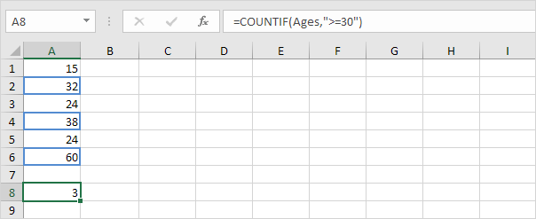
- Countif: The powerful COUNTIF function in Excel counts cells based on one criteria. This page contains many easy to follow COUNTIF examples.

- Count Blank/Nonblank Cells: This example shows you how to count blank and nonblank cells in Excel.
- Count Characters: Use the LEN function to count characters in Excel. Use LEN and SUBSTITUTE to count specific characters in Excel.
- Not Equal To: In Excel, <> means not equal to. The <> operator in Excel checks if two values are not equal to each other. Let's take a look at a few examples.
- Count Cells with Text: This page illustrates multiple ways to count cells with text in Excel. Visit our page about the COUNTIF function to count cells that contain specific text.
- Sum: Use the SUM function in Excel to sum a range of cells, an entire column or non-contiguous cells. You can also use AutoSum to quickly add a total row and a total column.

- Running Total: This page teaches you how to create a running total (cumulative sum) in Excel. A running total changes each time new data is added to a list.
- Sumif: The powerful SUMIF function in Excel sums cells based on one criteria. This page contains many easy to follow SUMIF examples.
- Sumproduct: To calculate the sum of the products of corresponding numbers in one or more ranges, use Excel's powerful SUMPRODUCT function.
2. Logical
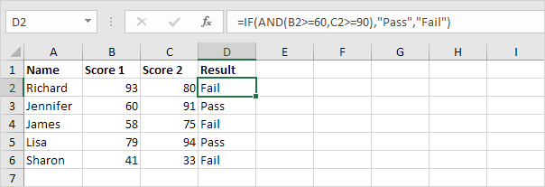
- If: The IF function is one of the most used functions in Excel. This page contains many easy to follow IF examples.

- Comparison Operators: Use comparison operators in Excel to check if two values are equal to each other, if one value is greater than another value, etc.
- Or: The OR function in Excel returns TRUE if any of the conditions are true and returns FALSE if all conditions are false. Combine the OR function with other functions and become an Excel expert.
- Roll the Dice: This example teaches you how to simulate the roll of two dice in Excel. If you are in a hurry, simply download the Excel file.
- Ifs: Use the IFS function in Excel 2016 or later when you have multiple conditions to meet. The IFS function returns a value corresponding to the first TRUE condition.
- Contains Specific Text: To check if a cell contains specific text, use ISNUMBER and SEARCH in Excel. There's no CONTAINS function in Excel.

- Switch: The SWITCH function in Excel looks up a specified value in a list of values and returns the result corresponding to the first match found.
- If Cell is Blank: Use the IF function and an empty string in Excel to check if a cell is blank. Use IF and ISBLANK to produce the exact same result.
- Absolute Value: The ABS function in Excel returns the absolute value of a number. In other words: the ABS function removes the minus sign (-) from a negative number, making it positive.
- And: The AND function in Excel evaluates multiple conditions and returns TRUE only if all conditions are TRUE.
3. Cell References
- Copy a Formula: Simply use CTRL + c and CTRL + v to copy and paste a formula in Excel. Use the fill handle in Excel to quickly copy a formula to other cells.

- 3D-reference: A 3D-reference in Excel refers to the same cell or range on multiple worksheets. First, we'll look at the alternative.
- Name Box: You can use the name box in Excel to select a cell, range or named range. You can also use the name box to quickly create a named range (important).
- External References: An external reference in Excel is a reference to a cell or range of cells in another workbook.
- Hyperlinks: Use the 'Insert Hyperlink' dialog box in Excel to create a hyperlink to an existing file, a web page or a place in this document. You can also use the HYPERLINK function.
- Union and Intersect: This example illustrates how to use the union and intersect operators in Excel
- Percent Change: The percent change formula is used very often in Excel. For example, to calculate the Monthly Change and Total Change.

- Add a Column: To add a column in Excel, right-click the column letter and click Insert. When you insert a column or row, cell references update automatically.
- Absolute Reference: To create an absolute reference in Excel, add $ symbols to a cell or range reference. This locks the reference. When you copy a formula, an absolute reference never changes.
- Address: The ADDRESS function in Excel creates a cell reference as text, based on a given row and column number.
4. Date & Time
- DateDif: To calculate the number of days, months or years between two dates in Excel, use the DATEDIF function. The DATEDIF function has three arguments.
- Today's Date: To enter today's date in Excel, use the TODAY function. To enter the current date and time, use the NOW function.
- Date and Time Formats: Dates and times in Excel can be displayed in a variety of ways. To apply a Date or Time format, execute the following steps.
- Calculate Age: To calculate age in Excel, use the DATEDIF function and TODAY. You can also use the age formula to calculate a person’s exact age in years, months, and days.

- Time Difference: Calculating the difference between two times in Excel can be tricky. Times are handled internally as numbers between 0 and 1.
- Weekdays: Use WEEKDAY, NETWORKDAYS and WORKDAY to create cool weekday formulas in Excel. Are you ready to improve your Excel skills?
- Days until Birthday: To calculate the number of days until your birthday in Excel, execute the following steps.
- Last Day of the Month: To get the date of the last day of the month in Excel, use the EOMONTH (End of Month) function.
- Add or Subtract Time: Use the TIME function in Excel to add or subtract hours, minutes and seconds. To add up times in Excel, simply use the SUM function.

- Quarter: An easy formula that returns the quarter for a given date. There's no built-in function in Excel that can do this.
- Day of the Year: An easy formula that returns the day of the year for a given date. There's no built-in function in Excel that can do this.
- Days between Dates: To calculate the number of days between two dates in Excel, subtract the start date from the end date, use DAYS or use DATEDIF.
5. Text
- Separate Strings: To separate strings in Excel, use RIGHT, LEN, FIND and LEFT. If you're not a formula hero, use Flash Fill to split text strings in Excel.
- Count Words: Use TRIM, LEN, SUBSTITUTE and SUMPRODUCT in Excel to count words. For example, let's count how many times a specific word occurs in a cell. This trick is pretty cool.

- Text to Columns: To separate the contents of one Excel cell into separate columns, you can use the 'Convert Text to Columns Wizard'.
- Find: Use the FIND function in Excel to find the position of a substring in a string. The FIND function is case-sensitive.
- Search: Use the SEARCH function in Excel to find the position of a substring in a string. The SEARCH function is case-insensitive and supports wildcards.
- Change Case: To change the case of text in Excel, use LOWER, UPPER or PROPER. If you're not a formula hero, use Flash Fill to change case in Excel.
- Remove Spaces: The TRIM function in Excel removes leading spaces, extra spaces and trailing spaces. Use the SUBSTITUTE function to remove all spaces or non-breaking spaces.

- Compare Text: This example shows two ways to compare text strings in Excel. One is case-sensitive and one is case-insensitive.
- Substitute vs Replace: If you know the text to be replaced, use the SUBSTITUTE function in Excel. If you know the position of the text to be replaced, use the REPLACE function.
- Text: When joining text and a number, use the TEXT function in Excel to format that number. This page contains many easy to follow TEXT function examples.
- Concatenate: Use CONCATENATE, CONCAT, TEXTJOIN or the & operator in Excel to concatenate (join) two or more text strings.

- Substring: There's no SUBSTRING function in Excel. Use MID, LEFT, RIGHT, FIND, LEN, SUBSTITUTE, REPT, TRIM and MAX in Excel to extract substrings.
6. Lookup & Reference
- Vlookup: The VLOOKUP function is one of the most popular functions in Excel. This page contains many easy to follow VLOOKUP examples.

- Tax Rates: This example teaches you how to calculate the tax on an income using the VLOOKUP function in Excel.
- Index and Match: Use INDEX and MATCH in Excel and impress your boss. Instead of using VLOOKUP, use INDEX and MATCH. To perform advanced lookups, you'll need INDEX and MATCH.
- Two-way Lookup: To lookup a value in a two-dimensional range, use INDEX and MATCH in Excel.
- Offset: The OFFSET function in Excel returns a cell or range of cells that is a specified number of rows and columns from a cell or range of cells.
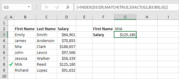
- Case-sensitive Lookup: By default, the VLOOKUP function performs a case-insensitive lookup. However, you can use INDEX, MATCH and EXACT in Excel to perform a case-sensitive lookup.

- Left Lookup: The VLOOKUP function only looks to the right. To look up a value in any column and return the corresponding value to the left, simply use INDEX and MATCH.
- Locate Maximum Value: To find the maximum value in Excel, use the MAX function. To find the cell address of the maximum value in a column, use MAX, MATCH and ADDRESS.
- Indirect: Use the INDIRECT function in Excel to convert a text string into a valid reference. You can use the & operator to create text strings.
- Two-column Lookup: This example teaches you how to perform a two-column lookup in Excel.
- Closest Match: To find the closest match to a target value in a data column, use INDEX, MATCH, ABS and MIN in Excel. Use the VLOOKUP function in Excel to find an approximate match.
- Compare Two Columns: To compare two columns, use IF, ISERROR and MATCH in Excel. You can display the duplicates or the unique values.
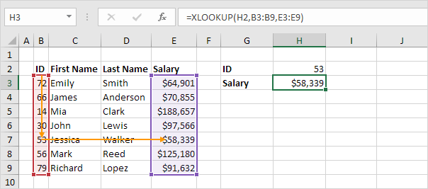
- Xlookup: If you have Excel 365 or Excel 2021, use XLOOKUP instead of VLOOKUP. The XLOOKUP function is easier to use and has some additional advantages.

- Xmatch: The XMATCH function in Excel enhances the MATCH function by adding new features, making it ideal for finding the position of items within arrays or cell ranges.
7. Financial
- PMT: The PMT function in Excel calculates the payment for a loan based on constant payments and a constant interest rate. This page contains many easy to follow PMT examples.
- Loans with Different Durations: This example teaches you how to compare loans with different durations in Excel.
- Investment or Annuity: This example teaches you how to calculate the future value of an investment or the present value of an annuity.
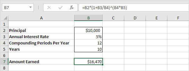
- Compound Interest: What's compound interest and what's the formula for compound interest in Excel? This example gives you the answers to these questions.

- CAGR: There's no CAGR function in Excel. However, simply use the RRI function in Excel to calculate the compound annual growth rate (CAGR) of an investment over a period of years.
- Loan Amortization Schedule: This example teaches you how to create a loan amortization schedule in Excel.
- NPV: The correct NPV formula in Excel uses the NPV function to calculate the present value of a series of future cash flows and subtracts the initial investment.
- IRR: Use the IRR function in Excel to calculate a project's internal rate of return. The internal rate of return is the discount rate that makes the net present value equal to zero.
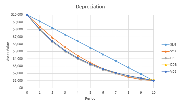
- Depreciation: Excel offers five different depreciation functions. We consider an asset with an initial cost of $10,000, a salvage value (residual value) of $1000 and a useful life of 10 periods (years).

- Profit Margin: Calculating gross profit margin, operating profit margin and net profit margin in Excel is easy. Simply use the formulas explained on this page.
8. Statistical
- Average: The AVERAGE function in Excel calculates the average (arithmetic mean) of a group of numbers.
- Negative Numbers to Zero: A clever Excel trick to change negative numbers to zero but leave positive numbers unchanged.
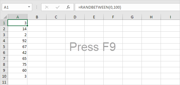
- Random Numbers: Excel has two very useful functions when it comes to generating random numbers. RAND and RANDBETWEEN.

- Rank: The RANK function in Excel returns the rank of a number in a list of numbers. Use RANK.AVG to return the average rank if more than one number has the same rank.
- Percentiles and Quartiles: This example teaches you how to use PERCENTILE and QUARTILE in Excel.
- Box and Whisker Plot: This example teaches you how to create a box and whisker plot in Excel. A box and whisker plot shows the minimum value, first quartile, median, third quartile and maximum value of a data set.
- AverageIf: The AVERAGEIF function in Excel calculates the average of cells that meet one criteria. AVERAGEIFS calculates the average of cells that meet multiple criteria.
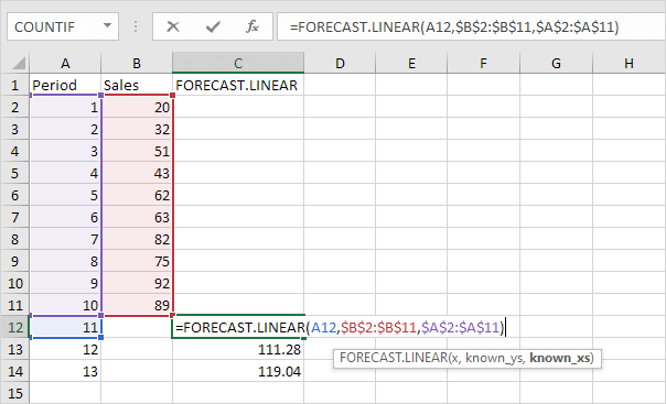
- Forecast: The FORECAST.LINEAR function in Excel predicts a future value along a linear trend. The FORECAST.ETS function in Excel predicts a future value using Exponential Triple Smoothing, which takes into account seasonality.

- MaxIfs and MinIfs: Use MAXIFS and MINIFS in Excel 2016 or later to find the maximum and minimum value based on one criteria or multiple criteria.
- Weighted Average: To calculate a weighted average in Excel, simply use SUMPRODUCT and SUM.
- Mode: Use the MODE function in Excel to find the most frequently occurring number in a list of numbers. Use MODE.MULT to find multiple modes.
- Standard Deviation: This page explains how to calculate the standard deviation based on the entire population using the STDEV.P function in Excel and how to estimate the standard deviation based on a sample using the STDEV.S function in Excel.
- Frequency: The FREQUENCY function in Excel calculates how often values occur within the ranges you specify in a bin table.
9. Round
- Chop off Decimals: This example illustrates two functions to chop off decimals in Excel. INT and TRUNC.
- Nearest Multiple: This example illustrates three functions to round numbers to a multiple of x in Excel. MROUND, CEILING and FLOOR.

- Even and Odd: Use EVEN and ODD in Excel to round numbers. Use ISEVEN or ISODD in Excel to determine if a number is even or odd.
- Mod: The MOD function in Excel gives the remainder of a division. You can use the MOD (Modulus) function to determine whether a number is divisible by another number or to check if a number is even or odd.
- Rounding Times: Use MROUND in Excel to round a time to the nearest 15 minutes, the nearest 30 minutes, the nearest hour, etc.
10. Formula Errors
- IfError: Use the IFERROR function in Excel to return an alternative result, such as text, when a formula evaluates to an error.
- IsError: This example illustrates the ISERROR function in Excel.
- Aggregate: Excel functions such as SUM, COUNT, LARGE and MAX don't work if a range includes errors. However, you can easily use the AGGREGATE function to fix this.
- Circular Reference: A circular reference in Excel occurs when a formula directly or indirectly refers to its own cell. This is not possible.

- Formula Auditing: Formula auditing in Excel allows you to display the relationship between formulas and cells. The example below helps you master Formula Auditing quickly and easily.
- Sum Range with Errors: This example shows you how to create an array formula that sums a range with errors. You can also use the AGGREGATE function to sum a range with errors.
- Floating Point Errors: Excel stores and calculates floating point numbers. Sometimes, the result of a formula is a very close approximation.
- IFNA: Use the IFNA function in Excel to replace a #N/A error with a friendly message. The IFNA function only catches #N/A errors.
11. Array Formulas
- Count Errors: This example shows you how to create an array formula that counts the number of errors in a range.
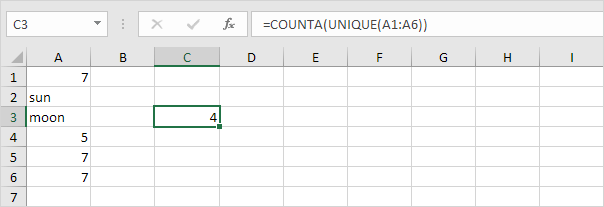
- Count Unique Values: This example shows you how to create an array formula that counts unique values. Use COUNTA and UNIQUE to count unique values in Excel 365/2021.

- Count with Or Criteria: Counting with Or criteria in Excel can be tricky. This article shows several easy to follow examples.
- Sum Every Nth Row: This example shows you how to create an array formula that sums every nth row in Excel. We will show it for n = 3, but you can do this for any number.
- Sum Largest Numbers: To sum the largest numbers in an Excel range, create an array formula or simply combine the SUMIF function with the LARGE function.
- Sum with Or Criteria: Summing with Or criteria in Excel can be tricky. This article shows several easy to follow examples.
- Most Frequently Occurring Word: This example teaches you how to find the most frequently occurring word in Excel.
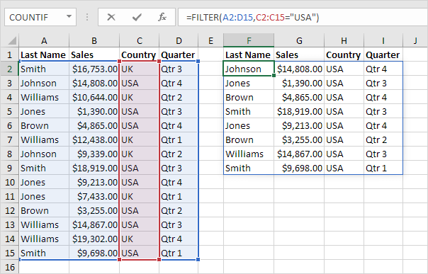
- Dynamic Arrays: Dynamic array formulas, entered into a single cell, fill multiple cells. This behavior in Excel 365/2021 is called spilling.

- LET function: Use the LET function in Excel 365/2021 to declare variables and assign values (or calculation results) to variables. Next, use these variables in a calculation.
- Array Manipulation: Use the new array manipulation functions in Excel 365 to quickly combine, shape and resize arrays.
- Lambda: Use LAMBDA and the Name Manager in Excel to create your own Excel function. You can use this custom function like any other Excel function!
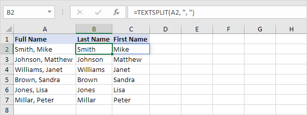
- TextSplit: Use the TEXTSPLIT function in Excel 365 to split text into rows or columns using delimiters.

Visit our next section: Data Analysis.
