SUMIF function in Excel

The powerful SUMIF function in Excel sums cells based on one criteria. This page contains many easy to follow SUMIF examples.

Numeric Criteria

Use the SUMIF function in Excel to sum cells based on numbers that meet specific criteria.

1. The SUMIF function below (two arguments) sums values in the range A1:A5 that are less than or equal to 10.

2. The following SUMIF function gives the exact same result. The & operator joins the 'less than or equal to' symbol and the value in cell C1.

3. The SUMIF function below (three arguments, last argument is the range to sum) sums values in the range B1:B5 if the corresponding cells in the range A1:A5 contain the value 25.

4. The following SUMIF function gives the exact same result (second argument refers to cell D1).

Text Criteria

Use the SUMIF function in Excel to sum cells based on text strings that meet specific criteria. Always enclose text in double quotation marks.

1. The SUMIF function below sums values in the range B1:B5 if the corresponding cells in the range A1:A5 contain exactly circle.

2. The SUMIF function below sums values in the range B1:B5 if the corresponding cells in the range A1:A5 do not contain exactly triangle.

3. The SUMIF function below sums values in the range B1:B5 if the corresponding cells in the range A1:A5 contain exactly circle + 1 character. A question mark (?) matches exactly one character.

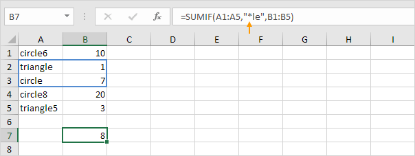
4. The SUMIF function below sums values in the range B1:B5 if the corresponding cells in the range A1:A5 contain a series of zero or more characters + le. An asterisk (*) matches a series of zero or more characters.

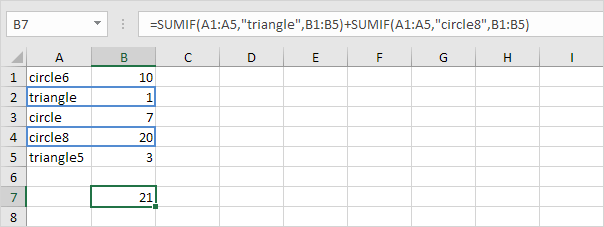
5. The SUMIF functions below sum values in the range B1:B5 if the corresponding cells in the range A1:A5 contain exactly triangle or circle8.

Date Criteria

Use the SUMIF function in Excel to sum cells based on dates that meet specific criteria.

1. The SUMIF function below sums the sales after January 20th, 2018.

Note: the DATE function in Excel accepts three arguments: year, month and day.

2. The SUMIF function below sums today's sales.

Note: today is August 3rd, 2018.

3. The SUMIFS function (with the letter S at the end) below sums the sales between two dates.

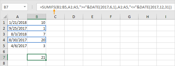
Note: the SUMIFS function in Excel sums cells based on two or more criteria (first argument is the range to sum, followed by two or more range/criteria pairs). Adjust the dates to sum the sales in a specific month, year, etc.

And Criteria

Summing with And criteria in Excel is easy.

1. For example, to sum the cells that meet the following criteria: Google and Stanford (two criteria ranges), simply use the SUMIFS function (with the letter S at the end).

Note: remember, when using the SUMIFS function, the first argument is the range to sum, followed by two or more range/criteria pairs.

Or Criteria

Summing with Or criteria in Excel can be tricky.

1. The formula below sums the cells that meet the following criteria: Google or Facebook (one criteria range). No rocket science so far.

2. However, if you want to sum the cells that meet the following criteria: Google or Stanford (two criteria ranges), you cannot simply use the SUMIF function twice (see the picture below).

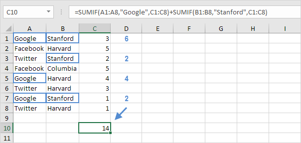
Note: cells that meet the criteria Google and Stanford are added twice, but they should only be added once. 10 is the answer we are looking for.

3. The array formula below does the trick.

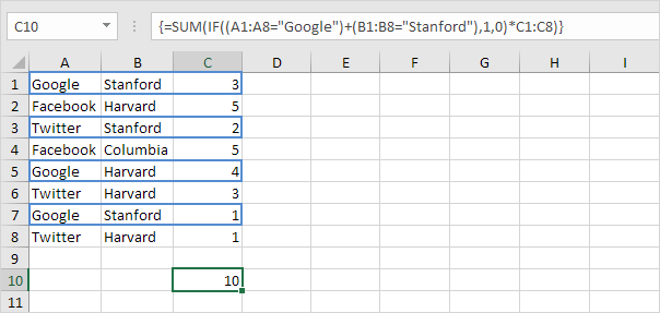
Note: finish an array formula by pressing CTRL + SHIFT + ENTER. Excel adds the curly braces {}. In Excel 365 or Excel 2021, finish by simply pressing Enter. You won't see curly braces. Visit our page about Summing with Or Criteria for instructions on how to create this array formula.