RANK function in Excel

The RANK function in Excel returns the rank of a number in a list of numbers. Use RANK.AVG to return the average rank if more than one number has the same rank.

1. If the third argument is omitted (or 0), Excel ranks the largest number first, second largest number second, etc.

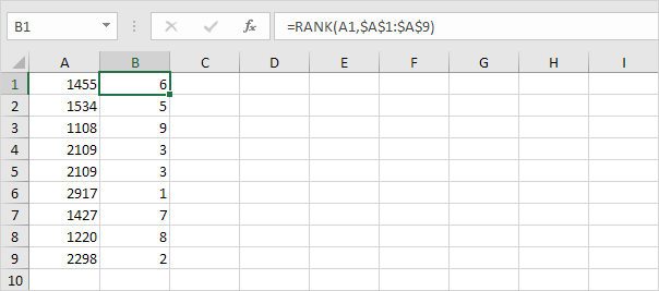
Note: when we drag this formula down, the absolute reference ($A$1:$A$9) stays the same, while the relative reference (A1) changes to A2, A3, A4, etc.

2. If the third argument is 1, Excel ranks the smallest number first, second smallest number second, etc.

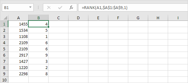
Note: the RANK function is an old function. Microsoft Excel recommends using the new RANK.EQ function in Excel 2010 or later. There's no difference at all between these two functions.

3. The RANK.AVG function in Excel 2010 or later returns the average rank if more than one number has the same rank.

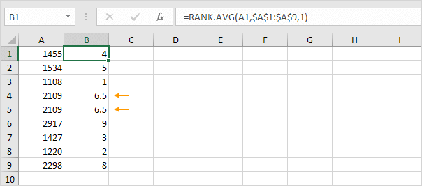
4. To create a clean RANK function, use a named range instead of an absolute range reference.

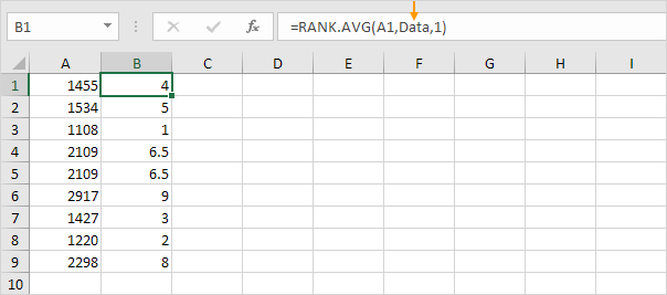
Explanation: the named range Data refers to the range A1:A9.

If you're using Excel 365 or Excel 2021, create the following RANK formula. This formula will amaze and impress your co-workers.

5. We want to show the top 3 results. Enter the value 3 into cell D2.

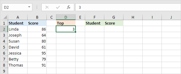
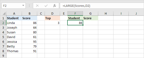
6. To find the third largest score, use the LARGE function below. The named range Scores refers to the range B2:B8.

7. The FILTER function below shows all students with a score greater than or equal to the third largest score.

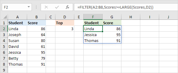
Note: the FILTER function, entered into cell F2, fills multiple cells. Wow!

8. Finally, add the SORT function to sort by the second column (second argument), in descending order (third argument).

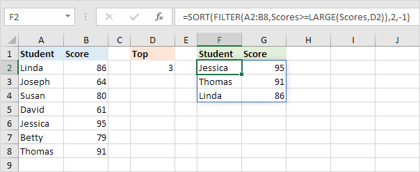
Note: use 1 to sort in ascending order, use -1 to sort in descending order.

9. This RANK formula works for every N. For example, enter the value 5 into cell D2 to show the top 5 results.

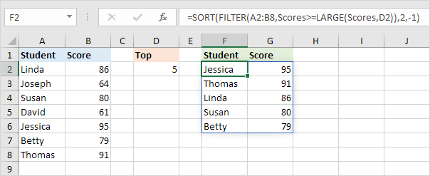
Note: this dynamic array formula, entered into cell F2, fills multiple cells. This behavior in Excel 365/2021 is called spilling. Tip: download the Excel file (right side of this page) and give it a try.