Become an Excel pro! 🚀 You can find many related examples and features on the right side of each chapterat the bottom of each chapter. Check out 100 popular pages below.
1 Drop-down List: Drop-down lists in Excel are helpful if you want to be sure that users select an item from a list, instead of typing their own values.

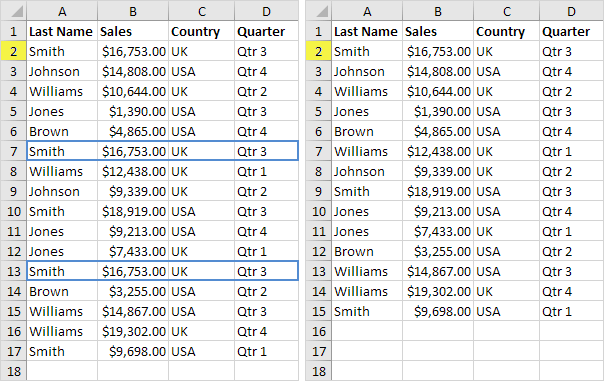
2 Find Duplicates: This page teaches you how to find duplicate values (or triplicates) and how to find duplicate rows in Excel.
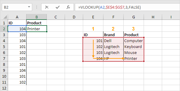
3 Vlookup: The VLOOKUP function is one of the most popular functions in Excel. This page contains many easy to follow VLOOKUP examples.
4 Histogram: This example teaches you how to make a histogram in Excel.
5 Regression: This example teaches you how to run a linear regression analysis in Excel and how to interpret the Summary Output.
6 Percent Change: The percent change formula is used very often in Excel. For example, to calculate the Monthly Change and Total Change.
7 Pareto Chart: A Pareto chart combines a column chart and a line graph. The Pareto principle states that, for many events, roughly 80% of the effects come from 20% of the causes.
8 Loan Amortization Schedule: This example teaches you how to create a loan amortization schedule in Excel.
9 Random Numbers: Excel has two very useful functions when it comes to generating random numbers. RAND and RANDBETWEEN.
10 If: The IF function is one of the most used functions in Excel. This page contains many easy to follow IF examples.
11 Remove Duplicates: This example teaches you how to remove duplicates in Excel.

12 Lock Cells: You can lock cells in Excel if you want to protect cells from being edited.
13 Standard Deviation: This page explains how to calculate the standard deviation based on the entire population using the STDEV.P function in Excel and how to estimate the standard deviation based on a sample using the STDEV.S function in Excel.
14 Count Unique Values: This example shows you how to create an array formula that counts unique values.
15 Gantt Chart: Excel does not offer Gantt as a chart type, but it's easy to create a Gantt chart by customizing the stacked bar chart type.
16 Countif: The powerful COUNTIF function in Excel counts cells based on one criteria. This page contains many easy to follow COUNTIF examples.
17 Budget: This example shows you how to create a budget in Excel. Follow this step-by-step guide and take control of your finances.
18 Line Chart: Line charts are used to display trends over time. Use a line chart if you have text labels, dates or a few numeric labels on the horizontal axis.
19 Transpose: Use the 'Paste Special Transpose' option to switch rows to columns or columns to rows in Excel. You can also use the TRANSPOSE function.
20 Compare Two Lists: This page describes how to compare two lists in Excel using conditional formatting and COUNTIF.
21 Sumif: The powerful SUMIF function in Excel sums cells based on one criteria. This page contains many easy to follow SUMIF examples.

22 Time Sheet: This example teaches you how to create a simple timesheet calculator in Excel.
23 Offset: The OFFSET function in Excel returns a cell or range of cells that is a specified number of rows and columns from a cell or range of cells.
24 Pie Chart: Pie charts are used to display the contribution of each value (slice) to a total (pie). Pie charts always use one data series.
25 Data Tables: Instead of creating different scenarios, you can create a data table to quickly try out different values for formulas. You can create a one variable data table or a two variable data table.
26 t-Test: This example teaches you how to perform a t-Test in Excel. The t-Test is used to test the null hypothesis that the means of two populations are equal.
27 Advanced Filter: This example teaches you how to apply an advanced filter in Excel to only display records that meet complex criteria.
28 Frequency Distribution: Did you know that you can use pivot tables to easily create a frequency distribution in Excel? You can also use the Analysis Toolpak to create a histogram.
29 Subtract: There's no SUBTRACT function in Excel. However, there are many ways to subtract numbers in Excel. Are you ready to improve your Excel skills?
30 Anova: This example teaches you how to perform a single factor ANOVA (analysis of variance) in Excel. A single factor or one-way ANOVA is used to test the null hypothesis that the means of several populations are all equal.
31 Correlation: We can use the CORREL function or the Analysis Toolpak add-in in Excel to find the correlation coefficient between two variables.

32 Compound Interest: What's compound interest and what's the formula for compound interest in Excel? This example gives you the answers to these questions.
33 Bar Chart: A bar chart is the horizontal version of a column chart. Use a bar chart if you have large text labels.
34 Concatenate: Use CONCATENATE, CONCAT, TEXTJOIN or the & operator in Excel to concatenate (join) two or more text strings.
35 Freeze Panes: If you have a large table of data in Excel, it can be useful to freeze rows or columns. This way you can keep rows or columns visible while scrolling through the rest of the worksheet.
36 Weighted Average: To calculate a weighted average in Excel, simply use SUMPRODUCT and SUM.
37 Index and Match: Use INDEX and MATCH in Excel and impress your boss. Instead of using VLOOKUP, use INDEX and MATCH. To perform advanced lookups, you'll need INDEX and MATCH.
38 Delete Blank Rows: This example teaches you how to delete blank rows or rows that contain blank cells.
39 Sumproduct: To calculate the sum of the products of corresponding numbers in one or more ranges, use Excel's powerful SUMPRODUCT function.
40 Merge Cells: Merge cells into one large cell to make clear that a label in Excel applies to multiple columns. Use CONCATENATE, TEXTJOIN or Flash Fill to merge cells without losing data.
41 Scatter Plot: Use a scatter plot (XY chart) to show scientific XY data. Scatter plots are often used to find out if there's a relationship between variables X and Y.

42 Percentage: Calculating percentages in Excel is easy. Percentage simply means 'out of 100', so 72% is '72 out of 100' and 4% is '4 out of 100', etc.
43 Contains Specific Text: To check if a cell contains specific text, use ISNUMBER and SEARCH in Excel. There's no CONTAINS function in Excel.
44 Pmt: The PMT function in Excel calculates the payment for a loan based on constant payments and a constant interest rate. This page contains many easy to follow PMT examples.
45 Calculate Age: To calculate age in Excel, use the DATEDIF function and TODAY. You can also use the age formula to calculate a person’s exact age in years, months, and days.
46 Wrap Text: Wrap text in Excel if you want to display long text on multiple lines in a single cell.
47 Indirect: Use the INDIRECT function in Excel to convert a text string into a valid reference. You can use the & operator to create text strings.
48 Multiply: To multiply numbers in Excel, use the asterisk symbol (*) or the PRODUCT function. Learn how to multiply columns and how to multiply a column by a constant.
49 Subtotal: Use the SUBTOTAL function in Excel instead of SUM, COUNT, MAX, etc. to ignore rows hidden by a filter or to ignore manually hidden rows.
50 Goal Seek: If you know the result you want from a formula, use Goal Seek in Excel to find the input value that produces this formula result.
51 Dynamic Arrays: Dynamic array formulas, entered into a single cell, fill multiple cells. This behavior in Excel 365/2021 is called spilling.

52 CAGR: There's no CAGR function in Excel. However, simply use the RRI function in Excel to calculate the compound annual growth rate (CAGR) of an investment over a period of years.
53 If Cell is Blank: Use the IF function and an empty string in Excel to check if a cell is blank. Use IF and ISBLANK to produce the exact same result.
54 Average: The AVERAGE function in Excel calculates the average (arithmetic mean) of a group of numbers.
55 Substring: There's no SUBSTRING function in Excel. Use MID, LEFT, RIGHT, FIND, LEN, SUBSTITUTE, REPT, TRIM and MAX in Excel to extract substrings.
56 Sum: Use the SUM function in Excel to sum a range of cells, an entire column or non-contiguous cells.
57 Compare Two Columns: To compare two columns, use IF, ISERROR and MATCH in Excel. You can display the duplicates or the unique values.
58 Divide: There's no DIVIDE function in Excel. Simply use the forward slash (/) to divide numbers in Excel.
59 Remove Spaces: The TRIM function in Excel removes leading spaces, extra spaces and trailing spaces. Use the SUBSTITUTE function to remove all spaces or non-breaking spaces.
60 Move Columns: To move columns in Excel, use the shift key or use Insert Cut Cells. You can also change the order of all columns in one magic move.
61 Flash Fill: Flash fill is a great Excel tool. Learn how to use flash fill to automatically extract data, combine data, and much more.

62 Hide Columns or Rows: Sometimes it can be useful to hide columns or rows in Excel. Learn how to hide a column, unhide all columns, hide cells, and much more.
63 Check Mark: To insert a check mark symbol in Excel, simply press SHIFT + P and use the Wingdings 2 font. You can also insert a checkbox in Excel.
64 Insert Row: To quickly insert a row in Excel, select a row and use the shortcut CTRL SHIFT +.
65 Comparison Operators: Use comparison operators in Excel to check if two values are equal to each other, if one value is greater than another value, etc.
66 NPV: The correct NPV formula in Excel uses the NPV function to calculate the present value of a series of future cash flows and subtracts the initial investment.
67 Bullet Points: This page illustrates 4 ways to insert bullet points in Excel.
68 AverageIf: The AVERAGEIF function in Excel calculates the average of cells that meet one criteria. AVERAGEIFS calculates the average of cells that meet multiple criteria.
69 Box and Whisker Plot: This example teaches you how to create a box and whisker plot in Excel. A box and whisker plot shows the minimum value, first quartile, median, third quartile and maximum value of a data set.
70 Hyperlinks: Use the 'Insert Hyperlink' dialog box in Excel to create a hyperlink to an existing file, a web page or a place in this document. You can also use the HYPERLINK function.
71 Quick Analysis: Use the Quick Analysis tool in Excel to quickly analyze your data. Quickly calculate totals, quickly insert tables, quickly apply conditional formatting and more.

72 Shade Alternate Rows: To shade alternate rows in Excel, use conditional formatting or apply a table style. Coloring every other row makes it easier to read your data.
73 IRR: Use the IRR function in Excel to calculate a project's internal rate of return.
74 Time Difference: Calculating the difference between two times in Excel can be tricky. Times are handled internally as numbers between 0 and 1.
75 PDF: This page teaches you how to convert an Excel file to a PDF file.
76 Today's Date: To enter today's date in Excel, use the TODAY function. To enter the current date and time, use the NOW function.
77 Forecast: The FORECAST.LINEAR function in Excel predicts a future value along a linear trend. The FORECAST.ETS function in Excel predicts a future value using Exponential Triple Smoothing, which takes into account seasonality.
78 Slicers: Use slicers in Excel to quickly and easily filter pivot tables. Connect multiple slicers to multiple pivot tables to create awesome reports.
79 Split Cells: To split the contents of a cell into multiple cells, use the Text to Columns wizard, flash fill or formulas.
80 Calendar: This example describes how to create a calendar in Excel (2025 calendar, 2026 calendar, etc). If you are in a hurry, simply download the Excel file.
81 Sparklines: Sparklines in Excel are graphs that fit in one cell. Sparklines are great for displaying trends. Excel offers three sparkline types: Line, Column and Win/Loss.

82 Xlookup: If you have Excel 365, use XLOOKUP instead of VLOOKUP. The XLOOKUP function is easier to use and has some additional advantages.
83 Square Root: The square root of a number is a value that, when multiplied by itself, gives the number. The SQRT function in Excel returns the square root of a number.
84 Absolute Reference: To create an absolute reference in Excel, add $ symbols to a cell or range reference. This locks the reference. When you copy a formula, an absolute reference never changes.
85 Randomize List: This article teaches you how to randomize (shuffle) a list in Excel.
86 Circular Reference: A circular reference in Excel occurs when a formula directly or indirectly refers to its own cell. This is not possible.
87 Running Total: This page teaches you how to create a running total (cumulative sum) in Excel. A running total changes each time new data is added to a list.
88 AutoFit: You probably know how to change the width of a column in Excel, but do you also know how to automatically fit the widest entry in a column?
89 Dependent Drop-down Lists: This example describes how to create dependent drop-down lists in Excel.
90 Add or Subtract Time: Use the TIME function in Excel to add or subtract hours, minutes and seconds. To add up times in Excel, simply use the SUM function.
91 Pivot Chart: A pivot chart is the visual representation of a pivot table in Excel. Pivot charts and pivot tables are connected with each other.

92 Frequency: The FREQUENCY function in Excel calculates how often values occur within the ranges you specify in a bin table.
93 Trendline: This example teaches you how to add a trendline to a chart in Excel.
94 Not Equal To: In Excel, <> means not equal to. The <> operator in Excel checks if two values are not equal to each other. Let's take a look at a few examples.
95 Weekdays: Use WEEKDAY, NETWORKDAYS and WORKDAY to create cool weekday formulas in Excel. Are you ready to improve your Excel skills?
96 AutoFill: Use AutoFill in Excel to automatically fill a series of cells. This page contains many easy to follow AutoFill examples.
97 Entire Rows and Columns: This example teaches you how to select entire rows and columns in Excel VBA. Are you ready?
98 Combination Chart: A combination chart is a chart that combines two or more chart types in a single chart.
99 Copy a Formula: Simply use CTRL + c and CTRL + v to copy and paste a formula in Excel. Use the fill handle in Excel to quickly copy a formula to other cells.
100 Rank: The RANK function in Excel returns the rank of a number in a list of numbers. Use RANK.AVG to return the average rank if more than one number has the same rank.
Check out all 300 examples.

