Number and Text Filters in Excel

This example teaches you how to apply a number filter and a text filter to only display records that meet certain criteria.

1. Click any single cell inside a data set.

2. On the Data tab, in the Sort & Filter group, click Filter.

Arrows in the column headers appear.

Number Filter

To apply a number filter, execute the following steps.

1. Click the arrow next to Sales.

2. Click Number Filters (this option is available because the Sales column contains numeric data) and select Greater Than from the list.

3. Enter 10,000 and click OK.

Result: Excel only displays the records where Sales is greater than $10,000.

Note: you can also display records equal to a value, less than a value, between two values, the top x records, records that are above average, etc. The sky is the limit!

Text Filter

To apply a text filter, execute the following steps.

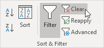
1. First, to remove the previously applied filter, on the Data tab, in the Sort & Filter group, click Clear.

2. Next, click the arrow next to Last Name.

3. Click Text Filters (this option is available because the Last Name column contains text data) and select Equals from the list.

4. Enter ?m* and click OK.

Note: a question mark (?) matches exactly one character. An asterisk (*) matches a series of zero or more characters.

Result: Excel only displays the records where the second character of Last Name equals m.

Note: you can also display records that begin with a specific character, end with a specific character, contain or do not contain a specific character, etc. The sky is the limit!