ANOVA in Excel

This example teaches you how to perform a single factor ANOVA (analysis of variance) in Excel. A single factor or one-way ANOVA is used to test the null hypothesis that the means of several populations are all equal.

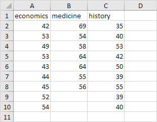
Below you can find the salaries of people who have a degree in economics, medicine or history.

H₀: μ₁ = μ₂ = μ₃
H₁: at least one of the means is different.

To perform a single factor ANOVA, execute the following steps.

1. On the Data tab, in the Analysis group, click Data Analysis.

Note: can't find the Data Analysis button? Click here to load the Analysis ToolPak add-in.

2. Select Anova: Single Factor and click OK.

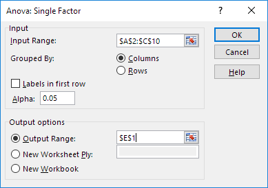
3. Click in the Input Range box and select the range A2:C10.

4. Click in the Output Range box and select cell E1.

5. Click OK.

Result:

Conclusion: if F > F crit, we reject the null hypothesis. This is the case, 15.196 > 3.443. Therefore, we reject the null hypothesis. The means of the three populations are not all equal. At least one of the means is different. However, the ANOVA does not tell you where the difference lies. You need a t-Test to test each pair of means.

If you're new here, welcome to Excel Easy! Join over 1 million monthly Excel learners. You can find popular courses here: Excel Functions and Data Analysis in Excel.